Tutorial 3: Using the Waveform Viewer
In this tutorial you will learn more about using the SIMetrix waveform viewer.
This tutorial is designed for version 8 and beyond of SIMetrix and SIMetrix/SIMPLIS, and all versions of SIMetrix/SIMPLIS Elements.
We continue on from the end of Tutorial 2: Creating a Schematic and Running a Simulation, which you should complete first if you are unfamiliar with running simulations. The schematic as completed from the end of tutorial 2 is provided.
Getting Started
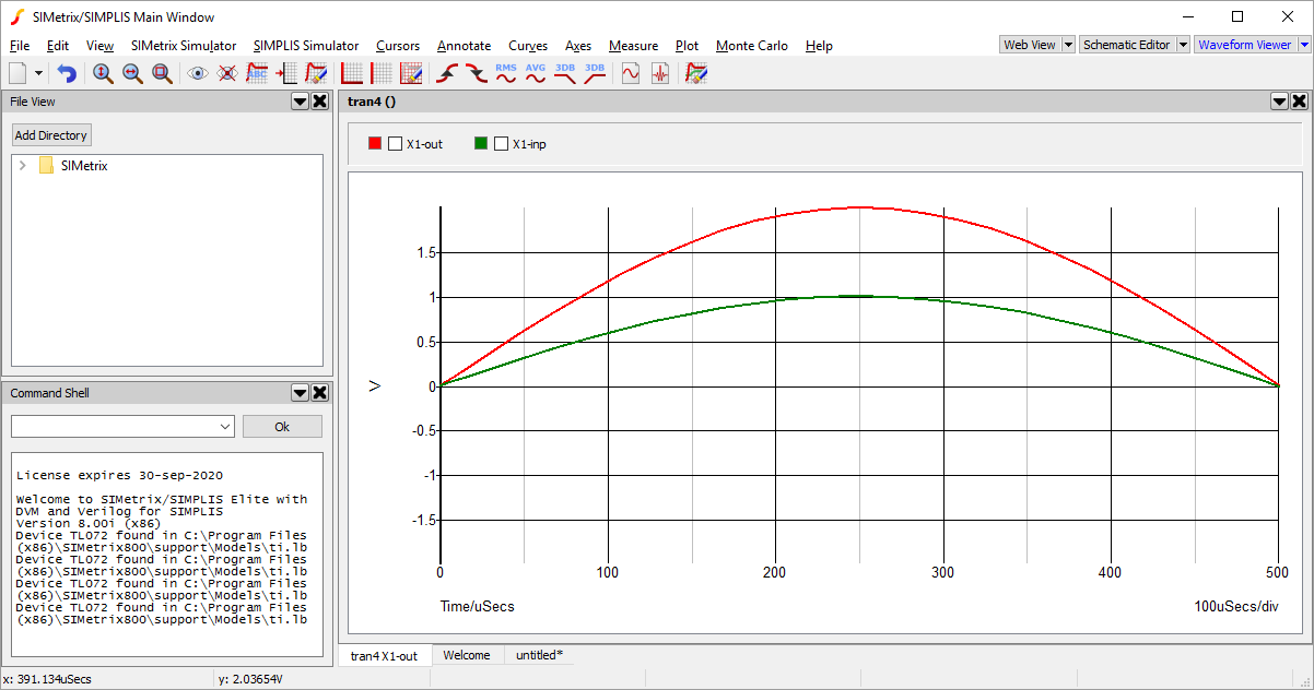
To begin, we will need the waveform output from the non-inverting amplifier that we developed in the previous tutorial. If you are continuing on from the previous tutorial, then you should already have the output and your SIMetrix workspace should look similar to the one below. If you are starting from this tutorial, download the schematic from above and run a simulation.
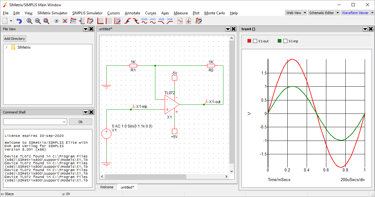
So that we can focus solely on the waveform, we will move the waveform panel so that it takes up the full workspace panel area. To do this, click and drag on the titlebar for the waveform (in our example pictures this has the title tran4(), but your title may appear with a different number and include a file path if you have saved your schematic previously). When you drag the panel a blue highlighted region will appear over the main workspace panel area, release the mouse in the blue highlighted region and the window will move there.
If when you release the waveform panel it opens up in a new window, open up the menu context panel by clicking on the down arrow in the panel title bar and choose the menu option (note the window name may appear differently depending on whether you are using SIMetrix, SIMetrix/SIMPLIS or SIMetrix/SIMPLIS Elements, but the name Main Window will remain). The waveform should now return to the main window and be docked in the position that we want it.
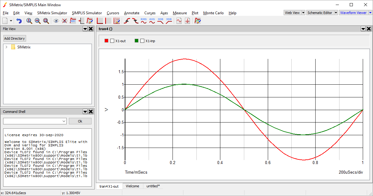
Your workspace should now look like the following:
Moving and Zooming
We will begin with a common requirement on viewing a waveform, adjusting what is being displayed on the screen by moving the view region and zooming in and out. Throughout we will use the default shortcut keys, but all operations can also be performed by using the appropriate menu option in the View menu.
 (shortcut key Home) will return the display so that the plotted waveforms all fit fully within the visible region.
To begin, we can move the areas we are viewing in the waveforms up, down, left and right, by using the keyboard cursor keys. We can zoom out by pressing F12 and zoom back in again by pressing Shift-F12. All of these movements are made by a fixed constant amount.
We can view a specific area of the waveform by clicking and dragging around the area that we want to view. When we click and drag on the waveform, a box will appear showing the region that will be displayed after releasing. This will adjust the movement and zoom automatically to show just that region. Remember to go back to the full waveform view, use the shortcut key Home.
To go back to the previous zoom or movement setting, you can use the Undo Zoom button  (shortcut Control-Z).
Measurements
The waveform viewer can provide certain measurements for plotted curves, such as RMS, frequency and minimum/maximum values, as appropriate.
First we need to select the curves that we want to receive the measurements for. Curves can be selected via the legend box that is above the waveform plot. The legend box, as shown below, displays all plotted curves, showing their colour, name and any measurements the have been made.

We are going to select both the X1-out and X1-inp curves. To do this, go to the legend box and click on the check boxes next to the names X1-out and X1-inp.
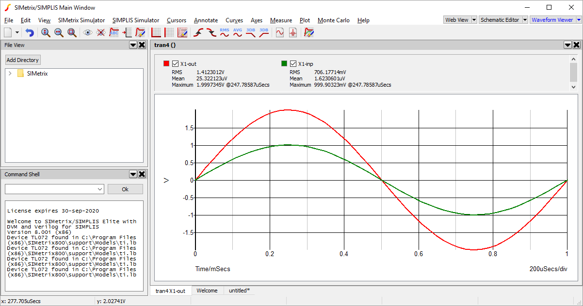
Next we will request the measurements for RMS, Mean and Maximum for these two curves. To do this, go to the menu and press the menu items for each of these measurements. The measurements will appear in the legend box, underneath the check box and name of the selected curves.
Your workspace should now look similar to the one below, with the measurements being displayed for the X1-out and X1-inp curves.
To remove the measurements, use menu . Alternately to remove specific measurements, make sure only a single curve is selected then use menu and choose the measurements to remove.
Cursors
Cursors provide a method of measuring the interval or difference between two points within a waveform window. They follow specific curves and allow markers to be positioned at specific points along a curve, with the difference between two markers being displayed.
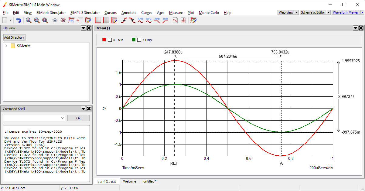
To turn on the cursors, use the menu . A pop-up box may appear, giving you brief instructions on cursor usage, which can be closed. Your workspace should now look similar to the one below.
Initially we are provided with two cursors, labelled REF and A, these labels can be found on the x-axis. The cursors are positioned at two points on a curve, the points are by default placed at the intersection of the vertical line going up from the label name and the horizontal line with the same line-style. The cursors are visually shown with a horizontal-vertical cross at this intersection.
The x and y values of the cursor positions are shown above the waveform for the x values and to the right of the waveform for the y values. The difference between the x and y cursor values are also shown in the same regions.
We can move the cursors along the x-axis, by moving the mouse pointer to one of the horizontal lines, where the mouse pointer will change to a horiztonal resize icon, then left clicking and dragging the cursor, moving it left or right. The cursor y value will follow the curve it is attached to. Similarly we can move along the y-axis by dragging one of the horiztonal cursor marker lines. This movement will be locked to the minimum and maximum values of the curve in the direction the cursor is being moved, or the maximum of the visible axis region, whichever is less. Dragging the cursor fully up, down, left or right, will move the cursor to the maximum extent on the curve, which may mean that the cursor appears to jump to another area of the curve if that area is the maximum or minimum as required.
Currently the cursors are both attached to the same curve. Now lets say we want to measure the voltage difference between the maximum of X1-out and the minimum of X1-inp. To do this we will need to move one of the cursors to the other curve. For this example we are assuming both cursors are currently attached to X1-out and we will move the A cursor to X1-inp. If your cursors are currently attached to a different curve, use the instructions below but ensure that REF is attached to X1-out and A is attached to X1-inp.
Move cursor A by placing the mouse pointer over the intersection point for cursor A. The mouse pointer should change to an icon showing arrows going up, down, left and right. Click and drag with the left mouse button when this icon is shown and move the mouse pointer to a point along the X1-inp curve and release the mouse button. The cursor should now snap to the X1-inp curve.
Next, to select the maximum of curve X1-out, move the REF cursor fully upwards by dragging the horiztonal cursor marker. Depending on product version, you may need to make minor adjustments to the x-position to get a maximum value. Similarly, move the A cursor fully down to get the minimum of the X1-inp curve. Your workspace should look similar to the following, showing a voltage difference of 3V.
Next we'll also measure the minimum of X1-out and compare this to the maximum of X1-out. Instead of moving our cursor A, we will add a new cursor, so then we can see the two difference measurements at the same time.
Use menu . A pop-up will display, shown below, asking for the definition of the new cursor.
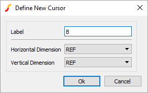
The cursor is defined with a label and cursor it is attached to when displaying the measurements on the horiztonal and vertical dimension. We want to use the default settings, which will give us a new cursor named B that will measure the difference between itself and the REF cursor. Press Ok to add the cursor.
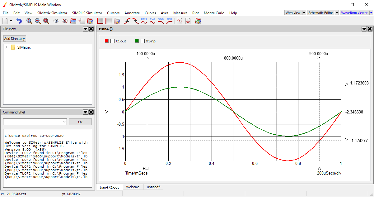
The new cursor will now appear on the waveform, you will most likely find it at the far left of the visible waveform area. As we did earilier, move this new cursor so that is at the lowest point of X1-out, you may need to change the curve that the cursor is attached to. Your workspace should now look like the one below.
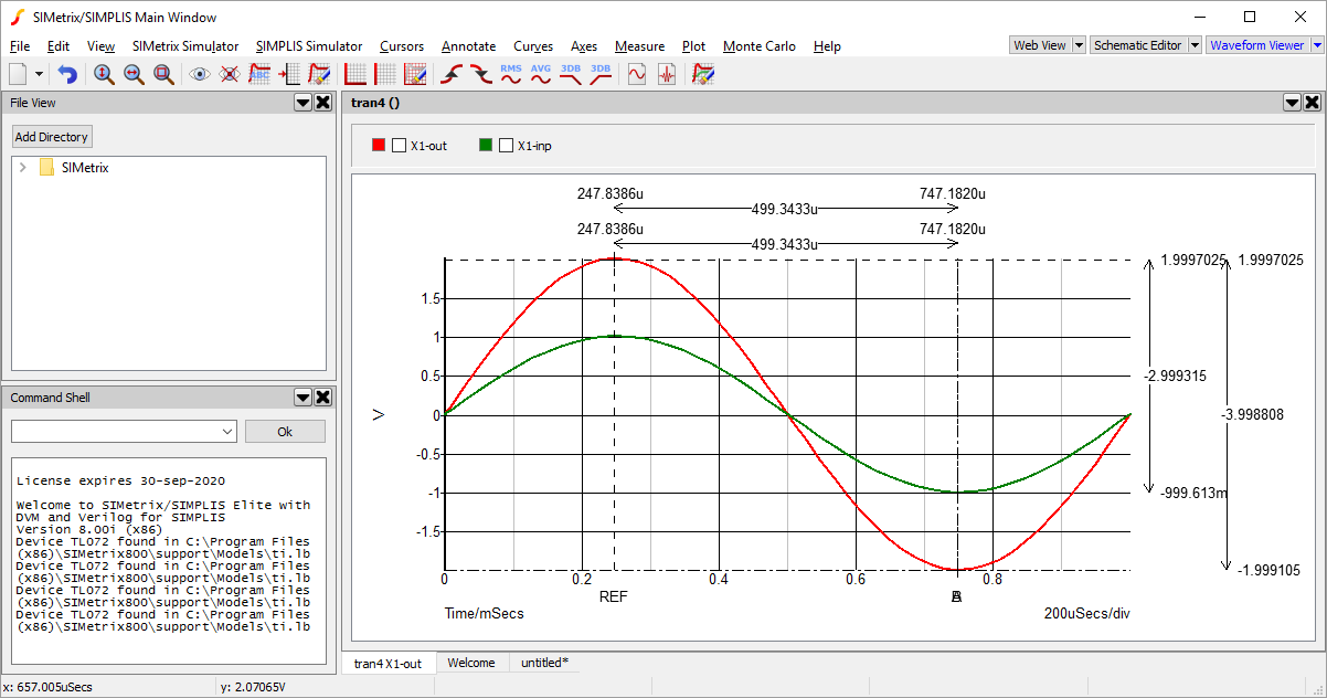
When multiple cursors are placed on the waveform, multiple measurement indicators are shown alongside the waveform. In this case it allows us to read-off the voltage differences between the two curves as 3V and 4V respectively.
To turn cursors off you can use menu , alternately to remove cursors that were added in addition to the two first cursors you can use the menu and choose the additional cursor to remove.
Axes
This section will cover some of basic operations that can be performed on axes. This will include adjusting the visible region of axes, handling additional y-axes and splitting curves up so each curve has it's own axis.
To begin we will adjust the visible limits on an axis. Use menu , a window will pop-up similar to the one below.
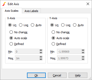
From here we adjust the limits used on the x and y axes, change the scale type and adjust the labels used. In this tutorial we are only going to adjust the axis limits. By default the axis limits are automatically derived from the data within the curves, as can be seen by the option Auto scale being selected for both the x-axis and the y-axis.
On the x-axis box, change the selection from Auto scale to Defined. The Min and Max fields will now become active for the x-axis. Adjust the Max value to 0.5m and press Ok. The waveform will now adjust so that the x-axis is between 0 and 500µs. If wanted, we can use the right cursor key to move along the x-axis and display more of the curve keeping the same level of zoom.
Reset the view using the shortcut key Home.
Next we will plot a curve that uses a different measurement unit. Using the tabs at the bottom of the waveform panel, switch back to the non-inverting amplifier schematic we used to generate this waveform from.
We are going to plot the current at the output of the op-amp. To do this, with the schematic visible and selected, use menu , the cursor will change to an icon of a probe. Click on the output pin of the op-amp. The view will automatically change back to the waveform viewer, where it will now have a third curve showing the current we selected, which should appear similar to the one below.
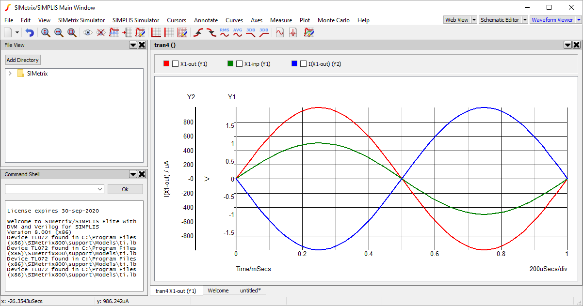
We can now see that a second y-axis has been added. Additionally, the y-axis being used by each curve is now also displayed in the legend box in brackets.
Previously, when we used the edit axis pop-up we were given options to adjust the x-axis and y-axis, which leaves some ambiguity over which y-axis would be adjusted now that we have more than one y-axis. We resolve this issue with the concept of a selected axis. The waveform viewer shows which y-axis is selected by highlighting one of the stacked y-axes. In the picture above Y2 is selected as it appers with bold highlighting. To change the selected axis, you just click on the y-axis that you want to select. Now when you use the edit axis menu, any changes requested on the y-axis will be made to the selected y-axis.
Next Steps
This tutorial has provided the basics of using the waveform viewer. Nearly all aspects of the waveform viewer have more advanced functionality, which can be learnt from the documentation.